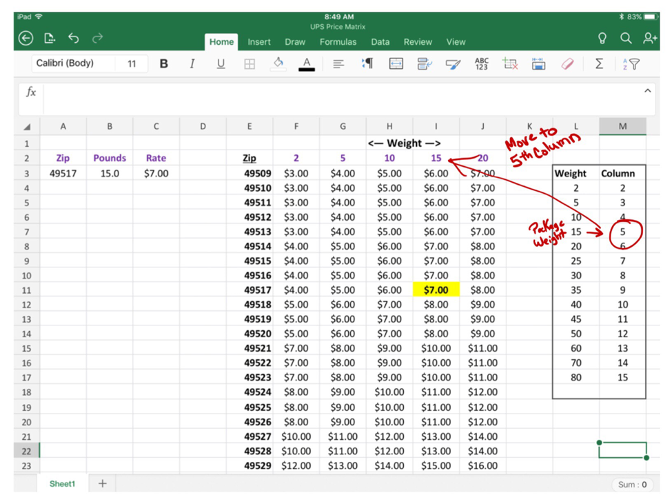
Most people who use VLOOKUPs stick to using it with only one variable. The vertical part is variable but the horizontal movement is fixed at a set number of columns.They might create a VLOOKUP to scan down a component parts list to grab the standard cost. The only variable is the item number. So the formula will look for that specific item number in a list and move over the designated number of columns to where the standard cost is.
But a lot of times, you may need to enter two variables. When I was working with the Cabela’s Corporation I created some complex Excel models to predict our delivery costs based on zip codes. But cost is linked to both zip code and weight. Therefore I needed two variables, distance and weight. My VLOOKUP needed to be able flex up and down based on zip code and left or right based on weight.
I used one VLOOKUP formula to look for the zip code and I had another VLookup formula nested within to look for the weight. This allowed the number of columns that Excel had to move to the right to be variable.
You can’t use the FALSE command if you are searching within a range so I left if off. Because if a package is between 11-15 pounds it will be the same price. So omitting the FALSE allows you to grab results by a range.
=VLookup(A3,E3:J30,5,FALSE)
I’m oversimplifying for brevity’s sake, so you’ll need to play around with it a bit to fit your needs. When Cabela’s was evaluating cities to place distribution centers, I was able to take historical package delivery costs and price that history out of other cities and come up with a delta to actual. This allowed me to quantify how much more or less we’d spend if we shifted volume to a different city. But this can be applied to any scenario where you need to pick a value from a table.
Bonus Tip
Don’t you hate it when you can’t sum a column because you have errors in there caused by divide by zero errors? Use IFERROR so that you don’t end up with lots of #DIV/0! type errors. Placing IFERROR in your formula’s will rid you of the dreaded #DIV/0! forever. You just need to do the following:
=IFERROR(your formula,0)
This formula sets a default action if it encounters any kind of error. That default action is defined after the comma. In this case, I want Excel to enter a 0. But you could also type a message by using quotes or enter a cell reference.
So there you go. That should keep you busy for a little while and before you know it you may be vying for a spot at the World Excel Championships.
Now available in iBooks ---> The Tesla Bubble


 RSS Feed